Housing Prices
This data is taken from Kaggle and concerns predicting housing prices. The problem of this dataset is tagged as a classification problem but clearly, the price field is continuous, and so this data is more naturally a regression problem. We have discretized the features as follows.
price: [low, medium, high]
area: [very_low, low, medium, high, very_high]
bedrooms: [low, medium, high]
bathrooms: [low, high]
stories: [low, medium, high]
parking, [low, medium, high]
The price and area features are discretized using univariate k-means clustering. The other features were binned using manual inspection (work omitted for brevity).
[1]:
import pandas as pd
import numpy as np
from sklearn.cluster import KMeans

def discretize(column, df, n_clusters=3):
    X = df[[column]]

    kmeans = KMeans(n_clusters=n_clusters, random_state=37)
    kmeans.fit(X)

    c2v = {c: v for v, (c, _) in list(enumerate(sorted(list(enumerate(np.ravel(kmeans.cluster_centers_))), key=lambda tup: tup[1])))}
    c2v

    y = pd.Series(kmeans.predict(X)).map(c2v)
    return y

df = pd.read_csv('./data/Housing.csv') \
    .assign(
        price=lambda d: discretize('price', d).map({0: 'low', 1: 'medium', 2: 'high'}),
        area=lambda d: discretize('area', d, 5).map({0: 'very_low', 1: 'low', 2: 'medium', 3: 'high', 4: 'very_high'}),
        bedrooms=lambda d: pd.cut(d['bedrooms'], [0, 2, 3, 10], include_lowest=True, labels=['low', 'medium', 'high']),
        bathrooms=lambda d: pd.cut(d['bathrooms'], [0, 1, 5], include_lowest=True, labels=['low', 'high']),
        stories=lambda d: pd.cut(d['stories'], [0, 1, 2, 5], include_lowest=True, labels=['low', 'medium', 'high']),
        parking=lambda d: d['parking'].map({0: 'low', 1: 'medium', 2: 'high', 3: 'high'})
    )
df.shape
[1]:
(545, 13)
[2]:
df.info()
<class 'pandas.core.frame.DataFrame'>
RangeIndex: 545 entries, 0 to 544
Data columns (total 13 columns):
 #   Column            Non-Null Count  Dtype
---  ------            --------------  -----
 0   price             545 non-null    object
 1   area              545 non-null    object
 2   bedrooms          545 non-null    category
 3   bathrooms         545 non-null    category
 4   stories           545 non-null    category
 5   mainroad          545 non-null    object
 6   guestroom         545 non-null    object
 7   basement          545 non-null    object
 8   hotwaterheating   545 non-null    object
 9   airconditioning   545 non-null    object
 10  parking           545 non-null    object
 11  prefarea          545 non-null    object
 12  furnishingstatus  545 non-null    object
dtypes: category(3), object(10)
memory usage: 44.7+ KB
Spark
Now let’s load up the data into a Spark dataframe.
[3]:
from pyspark.sql import SparkSession

spark = SparkSession \
    .builder \
    .appName('housing') \
    .master('local[*]') \
    .getOrCreate()

sdf = spark.createDataFrame(df).cache()
sdf.count()
Setting default log level to "WARN".
To adjust logging level use sc.setLogLevel(newLevel). For SparkR, use setLogLevel(newLevel).
23/09/10 17:42:06 WARN NativeCodeLoader: Unable to load native-hadoop library for your platform... using builtin-java classes where applicable
[3]:
545
[4]:
sdf.show(5)
+-----+----+--------+---------+-------+--------+---------+--------+---------------+---------------+-------+--------+----------------+
|price|area|bedrooms|bathrooms|stories|mainroad|guestroom|basement|hotwaterheating|airconditioning|parking|prefarea|furnishingstatus|
+-----+----+--------+---------+-------+--------+---------+--------+---------------+---------------+-------+--------+----------------+
| high|high|    high|     high|   high|     yes|       no|      no|             no|            yes|   high|     yes|       furnished|
| high|high|    high|     high|   high|     yes|       no|      no|             no|            yes|   high|      no|       furnished|
| high|high|  medium|     high| medium|     yes|       no|     yes|             no|             no|   high|     yes|  semi-furnished|
| high|high|    high|     high| medium|     yes|       no|     yes|             no|            yes|   high|     yes|       furnished|
| high|high|    high|      low| medium|     yes|      yes|     yes|             no|            yes|   high|      no|       furnished|
+-----+----+--------+---------+-------+--------+---------+--------+---------------+---------------+-------+--------+----------------+
only showing top 5 rows
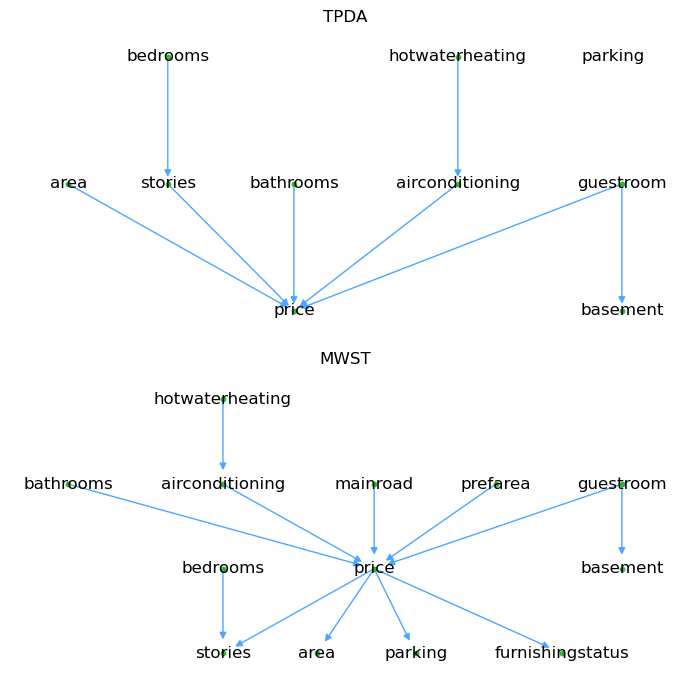
Learning
We will learn two models, one from Three-Phase Dependency Analysis (TPDA) and another from Maximum Weight Spanning Tree (MWST).
[5]:
from pysparkbbn.discrete.data import DiscreteData
from pysparkbbn.discrete.plearn import ParamLearner
from pysparkbbn.discrete.scblearn import Tpda, Mwst
from pysparkbbn.discrete.bbn import get_bbn
from pybbn.pptc.inferencecontroller import InferenceController

data = DiscreteData(sdf)

# TPDA
g_tpda = Tpda(data, cmi_threshold=0.05).get_network()
p_tpda = ParamLearner(data, g_tpda).get_params()
t_tpda = InferenceController.apply(get_bbn(g_tpda, p_tpda, data.get_profile()))

# MWST
g_mwst = Mwst(data).get_network()
p_mwst = ParamLearner(data, g_mwst).get_params()
t_mwst = InferenceController.apply(get_bbn(g_mwst, p_mwst, data.get_profile()))
23/09/10 17:42:10 WARN CacheManager: Asked to cache already cached data.
Here’s a plot of the structures learned.
[9]:
import networkx as nx
import matplotlib.pyplot as plt

pos_tpda = nx.nx_pydot.graphviz_layout(g_tpda, prog='dot')
pos_mwst = nx.nx_pydot.graphviz_layout(g_mwst, prog='dot')

fig, ax = plt.subplots(2, 1, figsize=(7, 7))
ax = np.ravel(ax)

nx.draw(
    g_tpda,
    pos_tpda,
    ax=ax[0],
    with_labels=True,
    node_size=10,
    node_color='#2eb82e',
    edge_color='#4da6ff',
    arrowsize=10,
    min_target_margin=5,
    nodelist=[n for n in g_tpda.nodes() if len(list(nx.to_undirected(g_tpda).neighbors(n))) > 0]
)

nx.draw(
    g_mwst,
    pos_mwst,
    ax=ax[1],
    with_labels=True,
    node_size=10,
    node_color='#2eb82e',
    edge_color='#4da6ff',
    arrowsize=10,
    min_target_margin=10,
    nodelist=[n for n in g_mwst.nodes() if len(list(nx.to_undirected(g_mwst).neighbors(n))) > 0]
)

ax[0].set_title('TPDA')
ax[1].set_title('MWST')

fig.tight_layout()
Lift
Now let’s see how the observation of each variable at its highest value gives lift to the housing price being high.
[7]:
from pybbn.graph.jointree import EvidenceBuilder

def get_sensitivity(name, value, tree):
    tree.unobserve_all()

    ev = EvidenceBuilder() \
        .with_node(tree.get_bbn_node_by_name(name)) \
        .with_evidence(value, 1.0) \
        .build()
    tree.set_observation(ev)

    meta = {'name': name, 'value': value}
    post = tree.get_posteriors()['price']

    return {**meta, **post}

n2v = {
    'bedrooms': 'high',
    'hotwaterheating': 'yes',
    'area': 'very_high',
    'stories': 'high',
    'bathrooms': 'high',
    'airconditioning': 'yes',
    'guestroom': 'yes',
    'basement': 'yes',
    'mainroad': 'yes',
    'parking': 'high',
    'prefarea': 'yes',
    'furnishingstatus': 'furnished'
}

t_tpda.unobserve_all()
h = t_tpda.get_posteriors()['price']['high']
m = t_tpda.get_posteriors()['price']['medium']
l = t_tpda.get_posteriors()['price']['low']

lift_df = pd.DataFrame([get_sensitivity(name, value, t_tpda) for name, value in n2v.items()]) \
    [['name', 'value', 'low', 'medium', 'high']] \
    .assign(
        low_lift=lambda d: d['low'] / l,
        medium_lift=lambda d: d['medium'] / m,
        high_lift=lambda d: d['high'] / h
    )
lift_df \
    .sort_values(['high_lift', 'medium_lift', 'low_lift'], ascending=False) \
    .rename(columns={
        'name': 'variable',
        'high_lift': 'price_lift'
    }) \
    [['variable', 'value', 'price_lift']]
[7]:
| variable | value | price_lift | |
|---|---|---|---|
| 2 | area | very_high | 3.945727 |
| 4 | bathrooms | high | 2.184265 |
| 5 | airconditioning | yes | 2.095619 |
| 3 | stories | high | 1.992604 |
| 0 | bedrooms | high | 1.389292 |
| 6 | guestroom | yes | 1.219085 |
| 7 | basement | yes | 1.043853 |
| 8 | mainroad | yes | 1.000000 |
| 9 | parking | high | 1.000000 |
| 10 | prefarea | yes | 1.000000 |
| 11 | furnishingstatus | furnished | 1.000000 |
| 1 | hotwaterheating | yes | 0.567470 |