Congressional Support

Let’s take a look at congressional data. This data is covers 5,000 legislative bills that were sponsored in Congress over 411 representatives (or the equivalent), 50 states (including some additional US territories) and 759 “subjects” (eg abortion, health, education, etc). In this notebook, we will use BBNs to estimate the lift of each state on sponsorship of a bill. We will also estimate the average causal effect (ACE) of states on subject sponsorship (eg what’s the ACE of California on sponsorship of abortion related legislative bills).

Initialize

Let’s load up the data, which has been transformed from its original “wide” form (each row is a legislative bill) to the “long” form below (each row is essentially a district’s sponsorship outcome).

[1]:

import pandas as pd
from pyspark.sql import SparkSession

def get_pdf(subject):
    f = (pdf.subject==subject)
    return pdf[f][['state', 'party', 'sponsor']]

def get_sdf(subject):
    pdf = get_pdf(subject)
    sdf = spark.createDataFrame(pdf)
    return sdf

spark = SparkSession \
    .builder \
    .appName('diabetes') \
    .master('local[*]') \
    .config('spark.executor.memory', '5g') \
    .config('spark.driver.memory', '10g') \
    .config('spark.memory.offHeap.enabled', 'true') \
    .config('spark.memory.offHeap.size', '5g') \
    .getOrCreate()

states = [
    'AL', 'AK', 'AZ', 'AR', 'CA', 'CO', 'CT',
    'DE', 'FL', 'GA', 'HI', 'ID', 'IL', 'IN',
    'IA', 'KS', 'KY', 'LA', 'ME', 'MD', 'MA',
    'MI', 'MN', 'MS', 'MO', 'MT', 'NE', 'NV',
    'NH', 'NJ', 'NM', 'NY', 'NC', 'ND', 'OH',
    'OK', 'OR', 'PA', 'RI', 'SC', 'SD', 'TN',
    'TX', 'UT', 'VT', 'VA', 'WA', 'WV', 'WI',
    'WY'
]

pdf = pd.read_csv('./data/congress-state-party-subject.csv', low_memory=False)
pdf = pdf[pdf['state'].isin(states)]

pdf.shape

Setting default log level to "WARN".
To adjust logging level use sc.setLogLevel(newLevel). For SparkR, use setLogLevel(newLevel).

23/09/12 01:22:52 WARN NativeCodeLoader: Unable to load native-hadoop library for your platform... using builtin-java classes where applicable

[1]:

(5600190, 6)

[2]:

pdf.head(10)

[2]:

	state	district	subject	legislation	party	sponsor
0	AK	AK_99	armed_forces_and_national_security	H.R. 4140	D	no
1	AL	AL_01	armed_forces_and_national_security	H.R. 4140	R	no
2	AL	AL_02	armed_forces_and_national_security	H.R. 4140	R	no
3	AL	AL_03	armed_forces_and_national_security	H.R. 4140	R	no
4	AL	AL_04	armed_forces_and_national_security	H.R. 4140	R	no
5	AL	AL_05	armed_forces_and_national_security	H.R. 4140	R	no
6	AL	AL_06	armed_forces_and_national_security	H.R. 4140	R	no
7	AL	AL_07	armed_forces_and_national_security	H.R. 4140	D	no
8	AR	AR_01	armed_forces_and_national_security	H.R. 4140	R	no
9	AR	AR_02	armed_forces_and_national_security	H.R. 4140	R	no

BBN

The code below are bootstrap code to build a BBN from the data so that we can estimate lift and ACE. All structures are composed of a triplet \((X, Y, Z)\) where

\(X \rightarrow Y\),
\(Z \rightarrow Y\), and
\(Z \rightarrow X\).

In these structures,

\(X\) is collection of states (eg all the 50 states when computing lift) or an individual state (eg CA, VA, MD, etc when estimating ACE),
\(Y\) is the sponsorship (yes or no), and
\(Z\) is the confounder and set to the party (eg replican R or democrat D).

Essentially, we want to know the impact of each state on sponsorship of legislative bill subjects.

[3]:

import networkx as nx
import matplotlib.pyplot as plt
from pysparkbbn.discrete.data import DiscreteData
from pysparkbbn.discrete.plearn import ParamLearner
from pysparkbbn.discrete.bbn import get_bbn
from pybbn.pptc.inferencecontroller import InferenceController

def get_structure(x='state', y='sponsor', z='party'):
    g = nx.DiGraph()

    g.add_node(x)
    g.add_node(z)
    g.add_node(y)

    g.add_edge(z, x)
    g.add_edge(z, y)
    g.add_edge(x, y)

    return g

def get_parameters(data, g):
    param_learner = ParamLearner(data, g)
    p = param_learner.get_params()
    return p

def get_jt(subject):
    d = DiscreteData(get_sdf(subject))
    g = get_structure()
    p = get_parameters(d, g)
    b = get_bbn(g, p, d.get_profile())
    t = InferenceController.apply(b)

    return d, g, p, b, t

def plot_structure(g):
    pos = nx.nx_pydot.graphviz_layout(g, prog='dot')

    fig, ax = plt.subplots(figsize=(3, 3))

    nx.draw(
        g,
        pos,
        ax=ax,
        with_labels=True,
        node_size=10,
        node_color='#2eb82e',
        edge_color='#4da6ff',
        arrowsize=10,
        min_target_margin=5
    )

    ax.set_title('Congressional Support')

    fig.tight_layout()

Lift

The states with the highest lift for the top 10 subjects (most frequently occuring subjects) are computed below.

[4]:

from pybbn.graph.jointree import EvidenceBuilder

def get_posterior(state, t, baseline_p):
    ev = EvidenceBuilder() \
        .with_node(t.get_bbn_node_by_name('state')) \
        .with_evidence(state, 1.0) \
        .build()

    t.unobserve_all()
    t.set_observation(ev)

    posterior = t.get_posteriors()['sponsor']
    lift = {
        'lift_no': posterior['no'] / baseline_p['no'],
        'lift_yes': posterior['yes'] / baseline_p['yes']
    }
    baseline = {
        'base_no': baseline_p['no'],
        'base_yes': baseline_p['yes']
    }
    posterior = {
        'post_no': posterior['no'],
        'post_yes': posterior['yes']
    }


    d = {'state': state}
    d = {**d, **baseline}
    d = {**d, **posterior}
    d = {**d, **lift}

    return d

def get_lift(t, subject):
    t.unobserve_all()
    baseline_p = t.get_posteriors()['sponsor']

    return pd.DataFrame([get_posterior(state, t, baseline_p) for state in pdf.state.unique()]) \
        .assign(subject=subject) \
        .sort_values(['lift_yes'], ascending=False) \
        .head(1)

def f(subject):
    *_, t = get_jt(subject)
    return get_lift(t, subject)

You can see that DE provides the highest lift for legislative bills associated with the “health” subject. The columns below are explained as follows.

state: the state (1 of 50) that generates the highest lift for sponsorship (yes)
base_no: the marginal percentage of no sponsorship,
base_yes: the marginal percentage of yes sponsorship,
post_no: the posterior probability of no sponsorship given the corresponding state,
post_yes: the posterior probability of yes sponsorship given the corresponding state,
lift_no: the lift of no sponsorship (eg base_no / post_no)
lift_yes: the lift of yes sponsorship (eg base_yes / post_yes)
subject: the legislative bill subject

[5]:

lift_df = pd.concat([f(subject) for subject in pdf.groupby(['subject']).size().sort_values(ascending=False).index[:10]])
lift_df

23/09/12 01:23:10 WARN GarbageCollectionMetrics: To enable non-built-in garbage collector(s) List(G1 Concurrent GC), users should configure it(them) to spark.eventLog.gcMetrics.youngGenerationGarbageCollectors or spark.eventLog.gcMetrics.oldGenerationGarbageCollectors

[5]:

	state	base_no	base_yes	post_no	post_yes	lift_no	lift_yes	subject
7	DE	0.962814	0.037186	0.873706	0.126294	0.907451	3.396263	health
25	MT	0.969950	0.030050	0.884615	0.115385	0.912021	3.839793	international_affairs
25	MT	0.975434	0.024566	0.870833	0.129167	0.892765	5.257993	government_operations_and_politics
29	NH	0.973497	0.026503	0.935252	0.064748	0.960714	2.443058	armed_forces_and_national_security
10	HI	0.954627	0.045373	0.925182	0.074818	0.969156	1.648946	crime_and_law_enforcement
10	HI	0.963228	0.036772	0.940476	0.059524	0.976380	1.618705	congressional_oversight
48	WV	0.970921	0.029079	0.938247	0.061753	0.966348	2.123622	taxation
25	MT	0.984835	0.015165	0.844538	0.155462	0.857542	10.251592	congress
10	HI	0.965579	0.034421	0.902703	0.097297	0.934882	2.826715	education
10	HI	0.962791	0.037209	0.921512	0.078488	0.957126	2.109375	government_information_and_archives

Average Causal Effect (ACE )

Now we will see the ACE of each state on sponsorship for selected subjects.

[6]:

from pybbn.causality.ace import Ace

def get_states(subject):
    return list(pdf.query(f'subject == "{subject}"')['state'].unique())

def get_ace(subject, state):
    d = pdf \
        .query(f'subject == "{subject}"') \
        .assign(**{
            state: lambda d: d['state'].apply(lambda s: 'yes' if s == state else 'no')
        }) \
        [[state, 'party', 'sponsor']]
    d = spark.createDataFrame(d)
    d = DiscreteData(d)

    g = get_structure(x=state, y='sponsor', z='party')
    p = get_parameters(d, g)
    b = get_bbn(g, p, d.get_profile())
    t = InferenceController.apply(b)

    a = Ace(b).get_ace(state, 'sponsor', 'yes')
    y = a['yes']
    n = a['no']
    diff = y - n

    return {
        'subject': subject,
        'state': state,
        'yes': y,
        'no': n,
        'ace': diff
    }

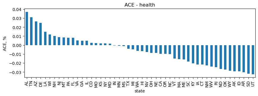
Health

As you can see below, AL has the highest, positive ACE on health legislative bills. UT actually has the highest, negative ACE on health bills.

[7]:

subject = 'health'
_df_health = pd.DataFrame([get_ace(subject, s) for s in get_states(subject)]) \
    .sort_values(['ace'], ascending=False) \
    .reset_index(drop=True)

[25]:

_ = _df_health.set_index(['state'])['ace'] \
    .plot(kind='bar', figsize=(10, 3), title='ACE - health', ylabel='ACE, %')

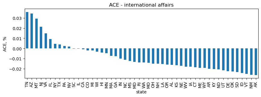
_images/use-case-congress-sponsorship_14_0.png

International affairs

TN ranks first with the highest, positive ACE on international affairs bills, and AK has the highest, negative ACE on these bills.

[8]:

subject = 'international_affairs'
_df_ia = pd.DataFrame([get_ace(subject, s) for s in get_states(subject)]) \
    .sort_values(['ace'], ascending=False) \
    .reset_index(drop=True)

[26]:

_ = _df_ia.set_index(['state'])['ace'] \
    .plot(kind='bar', figsize=(10, 3), title='ACE - international affairs', ylabel='ACE, %')

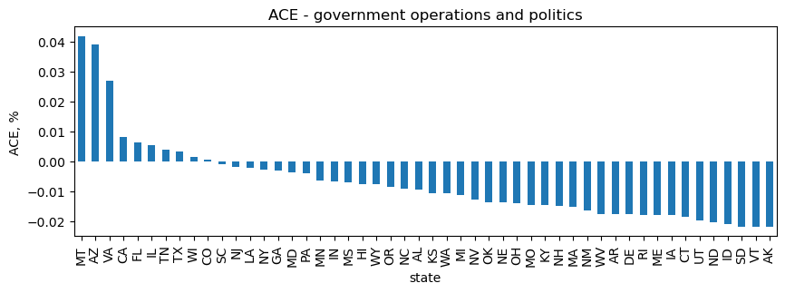
_images/use-case-congress-sponsorship_17_0.png

Government operations and politics

MT has the highest, positive ACE on government operations and politics bills, while AK has the highest, negative ACE.

[9]:

subject = 'government_operations_and_politics'
_df_gov_op = pd.DataFrame([get_ace(subject, s) for s in get_states(subject)]) \
    .sort_values(['ace'], ascending=False) \
    .reset_index(drop=True)

[27]:

_ = _df_gov_op.set_index(['state'])['ace'] \
    .plot(kind='bar', figsize=(10, 3), title='ACE - government operations and politics', ylabel='ACE, %')

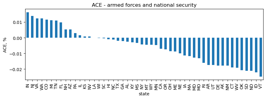
_images/use-case-congress-sponsorship_20_0.png

Armed forces and national security

For armed forces and national security, IN has the highest, positive ACE and VT has the highest, negative ACE.

[10]:

subject = 'armed_forces_and_national_security'
_df_afns = pd.DataFrame([get_ace(subject, s) for s in get_states(subject)]) \
    .sort_values(['ace'], ascending=False) \
    .reset_index(drop=True)

[28]:

_ = _df_afns.set_index(['state'])['ace'] \
    .plot(kind='bar', figsize=(10, 3), title='ACE - armed forces and national security', ylabel='ACE, %')

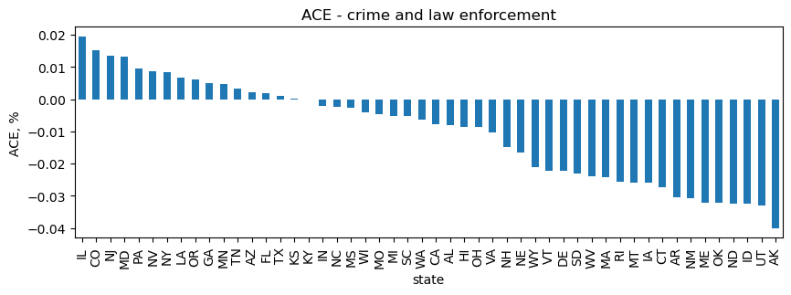
_images/use-case-congress-sponsorship_23_0.png

Crime and law enforcement

For crime and law enforcement, IL has the highest, positive ACE and AK has the highest, negative ACE.

[11]:

subject = 'crime_and_law_enforcement'
_df_cle = pd.DataFrame([get_ace(subject, s) for s in get_states(subject)]) \
    .sort_values(['ace'], ascending=False) \
    .reset_index(drop=True)

[29]:

_ = _df_cle.set_index(['state'])['ace'] \
    .plot(kind='bar', figsize=(10, 3), title='ACE - crime and law enforcement', ylabel='ACE, %')

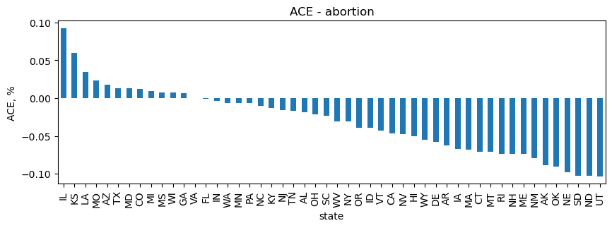
_images/use-case-congress-sponsorship_26_0.png

Abortion

For bills whose subjects include abortion, IL has the highest, positive ACE and UT, ND and SD have comparably the highest, negative ACE. It’s interesting to note that only 12 of 50 states have a positive ACE on abortion bill sponsorship.

[12]:

subject = 'abortion'
_df_abortion = pd.DataFrame([get_ace(subject, s) for s in get_states(subject)]) \
    .sort_values(['ace'], ascending=False) \
    .reset_index(drop=True)

[30]:

_ = _df_abortion.set_index(['state'])['ace'] \
    .plot(kind='bar', figsize=(10, 3), title='ACE - abortion', ylabel='ACE, %')

_images/use-case-congress-sponsorship_29_0.png