Constraint-Based

Constraint-based structure learning uses independence and conditional independence CI tests to constraint the relationships between nodes in a BBN.

Load data

Let’s read our data into a Spark DataFrame SDF.

sdf = spark.read.csv('hdfs://localhost/data-1479668986461.csv', header=True)
sdf.show()

+---+---+---+---+-----+
| n1| n2| n3| n4|   n5|
+---+---+---+---+-----+
|  f|  f|  f|  f|   no|
|  f|  t|  f|  f|   no|
|  f|  f|  f|  f|maybe|
|  f|  f|  f|  f|   no|
|  f|  f|  f|  t|  yes|
|  f|  f|  t|  t|  yes|
|  f|  f|  t|  t|   no|
|  t|  t|  t|  f|   no|
|  f|  f|  t|  t|maybe|
|  f|  f|  t|  t|maybe|
|  f|  f|  f|  t|maybe|
|  t|  f|  t|  t|maybe|
|  f|  f|  f|  t|maybe|
|  f|  t|  t|  t|  yes|
|  f|  f|  f|  t|maybe|
|  f|  t|  t|  t|maybe|
|  f|  f|  f|  f|   no|
|  t|  t|  t|  t|  yes|
|  f|  f|  t|  t|maybe|
|  f|  f|  f|  f|  yes|
+---+---+---+---+-----+
only showing top 20 rows

Discrete data

Now, we can build a data set using DiscreteData. The DiscreteData may be passed around to many different learning algorithms.

from pysparkbbn.discrete.data import DiscreteData

data = DiscreteData(sdf)

Constraint-based

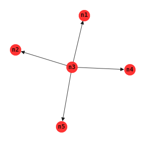
Naive Bayes

In the naive Bayes model, there is one class node and it has directed arcs going to all other nodes. The naive Bayes model is usually used for classification goals.

from pysparkbbn.discrete.scblearn import Naive

naive = Naive(data, 'n3')
g_naive = naive.get_network()

%matplotlib inline
import matplotlib.pyplot as plt
import networkx as nx

plt.style.use('ggplot')

fig, ax = plt.subplots(figsize=(5, 5))

nx.draw(g_naive,
        with_labels=True,
        node_size=500,
        alpha=0.8,
        font_weight='bold',
        font_family='monospace',
        node_color='r',
        arrowsize=15,
        ax=ax)

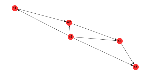
Tree augmented network

Tree augmented network TAN allows relationships between non-class nodes. This structure learning algorithm produces a network that is also typically used for classification goals.

from pysparkbbn.discrete.scblearn import Tan

tan = Tan(data, 'n3')
g_tan = tan.get_network()

fig, ax = plt.subplots(figsize=(10, 5))

nx.draw(g_tan,
        with_labels=True,
        node_size=500,
        alpha=0.8,
        font_weight='bold',
        font_family='monospace',
        node_color='r',
        arrowsize=15,
        ax=ax)

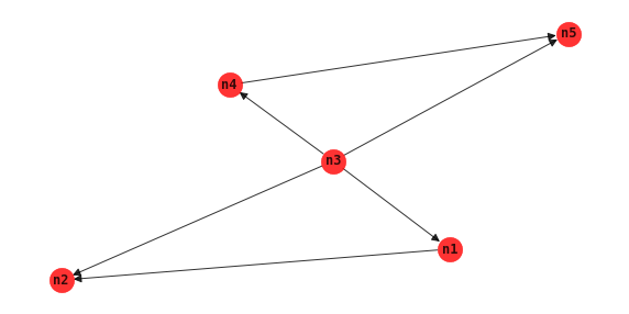
BN augmented naive Bayes

The BN augmented naive Bayes BAN algorithm is also used for classification tasks. This approach is similar to TAN, however, the independence and conditional independence tests always includes the class node in the conditioning set.

from pysparkbbn.discrete.scblearn import Ban

ban = Ban(data, 'n3', cmi_threshold=0.01, method='pc')
g_ban = ban.get_network()

fig, ax = plt.subplots(figsize=(10, 5))

nx.draw(g_ban,
        with_labels=True,
        node_size=500,
        alpha=0.8,
        font_weight='bold',
        font_family='monospace',
        node_color='r',
        arrowsize=15,
        ax=ax)

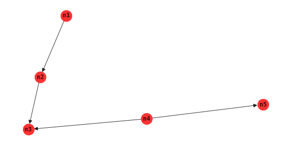
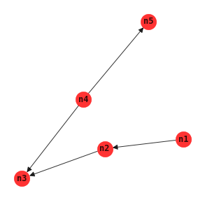
Maximum weight spanning tree

Assuming the distribution of the data comes from a tree distribution, then the maximum weight spanning tree MWST algorithm finds the BBN that maximizes the likelihood of the data.

from pysparkbbn.discrete.scblearn import Mwst

mwst = Mwst(data)
g_mwst = mwst.get_network()

fig, ax = plt.subplots(figsize=(5, 5))

nx.draw(g_mwst,
        with_labels=True,
        node_size=500,
        alpha=0.8,
        font_weight='bold',
        font_family='monospace',
        node_color='r',
        arrowsize=15,
        ax=ax)

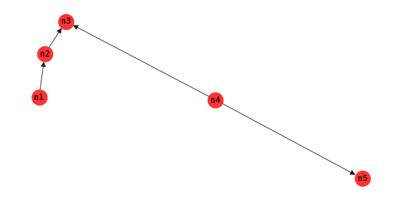
Three phase dependency analysis

Three phase dependency analysis TPDA uses three phases to learn a BBN structure.

• Drafting: creates a skeleton network structure using MWST.

• Thickening: adds nodes to the network structure using conditional independence tests.

• Thinning: removes nodes from the network structure using conditional independence tests.

from pysparkbbn.discrete.scblearn import Tpda

tpda = Tpda(data)
g_tpda = tpda.get_network()

fig, ax = plt.subplots(figsize=(10, 5))

nx.draw(g_tpda,
        with_labels=True,
        node_size=500,
        alpha=0.8,
        font_weight='bold',
        font_family='monospace',
        node_color='r',
        arrowsize=15,
        ax=ax)

PC algorithm

The PC algorithm starts with a fully connected graph and uses ever greater number of conditioning sets to remove edges.

from pysparkbbn.discrete.scblearn import Pc

pc = Pc(data)
g_pc = pc.get_network()

fig, ax = plt.subplots(figsize=(10, 5))

nx.draw(g_pc,
        with_labels=True,
        node_size=500,
        alpha=0.8,
        font_weight='bold',
        font_family='monospace',
        node_color='r',
        arrowsize=15,
        ax=ax)