Diabetes
Let’s work with a dataset from Kaggle. This dataset is about people with diabetes. There are 100,000 records over 8 features and 1 class label. There is severe class imbalance. We will use PySpark-BBN to learn two models–Naive Bayes (NB) and Maximum Weight Spanning Tree (MWST).
Load data
We will load the data using Pandas and also manipulate the data in Pandas before transferring the data to Spark. Note that continuous variables have been discretized as follows.
age
\([0, 12)\) to young
\([12, 18)\) to teen
\([18, 65)\) to adult
\([65, 100]\) to senior
bmi
\([0, 18.5)\) to underweight
\([18.5, 25)\) to normal
\([25, 30)\) to overweight
\([30, 35)\) to obesity_i
\([35, 40)\) to obesity_ii
\([40, 100]\) to obesity_iii
blood_glucose
\([0, 100)\) to normal
\([100, 200)\) to prediabetic
\([200, 500]\) to diabetic
hba1c
\([0, 5.7)\) to normal
\([5.7, 6.5)\) to prediabetic
\([6.5, 10]\) to diabetic
The following binary variables had 0 and 1 values and these values were transformed to no and yes, correspondingly.
hypertension
heart_disease
diabetes
Since there is class imbalance (there was a smaller number of people with diabetes than those without), we performed undersampling to combat the class imbalance. Lastly, records whose gender was not male or female (unspecified) were removed to combat data missingness issues.
[1]:
import pandas as pd

def get_data():
    cuts = {
        'age': [0, 12, 18, 65, 100],
        'bmi': [0, 18.5, 25, 30, 35, 40, 100],
        'blood_glucose': [0, 100, 200, 500],
        'hba1c': [0, 5.7, 6.5, 10]
    }
    labs = {
        'age': ['young', 'teen', 'adult', 'senior'],
        'bmi': ['underweight', 'normal', 'overweight', 'obesity_i', 'obesity_ii', 'obesity_iii'],
        'blood_glucose': ['normal', 'prediabetic', 'diabetic'],
        'hba1c': ['normal', 'prediabetic', 'diabetic']
    }

    pdf = pd.read_csv('./data/diabetes_prediction_dataset.csv') \
        .rename(columns={
            'smoking_history': 'smoking',
            'HbA1c_level': 'hba1c',
            'blood_glucose_level': 'blood_glucose'
        }) \
        .assign(
            gender=lambda d: d['gender'].str.lower(),
            age=lambda d: pd.cut(d['age'], cuts['age'], include_lowest=True, labels=labs['age']),
            hypertension=lambda d: d['hypertension'].map({0: 'no', 1: 'yes'}),
            heart_disease=lambda d: d['heart_disease'].map({0: 'no', 1: 'yes'}),
            smoking=lambda d: d['smoking'].apply(lambda s: s.lower().replace(' ', '_').strip()),
            bmi=lambda d: pd.cut(d['bmi'], cuts['bmi'], include_lowest=True, labels=labs['bmi']),
            hba1c=lambda d: pd.cut(d['hba1c'], cuts['hba1c'], include_lowest=True, labels=labs['hba1c']),
            blood_glucose=lambda d: pd.cut(d['blood_glucose'], cuts['blood_glucose'], labels=labs['blood_glucose']),
            diabetes=lambda d: d['diabetes'].map({0: 'no', 1: 'yes'})
        ) \
        .query('gender != "other"')

    # pos_df = pdf[pdf['diabetes']=='yes'].sample(n=pdf[pdf['diabetes']=='no'].shape[0], replace=True, random_state=37)
    # neg_df = pdf[pdf['diabetes']=='no']
    pos_df = pdf[pdf['diabetes']=='yes']
    neg_df = pdf[pdf['diabetes']=='no'].sample(n=pdf[pdf['diabetes']=='yes'].shape[0], replace=False, random_state=37)

    pdf = pd.concat([pos_df, neg_df]).reset_index(drop=True)

    return pdf

Xy = get_data()
X, y = Xy[Xy.columns.drop(['diabetes'])], Xy['diabetes']

Xy.shape, X.shape, y.shape
[1]:
((17000, 9), (17000, 8), (17000,))
Split data
The data was split into training tr and testing te folds using stratified shuffle splitting. We only take the training and testing fold from the first split.
[2]:
from sklearn.model_selection import StratifiedShuffleSplit


tr_index, te_index = next(StratifiedShuffleSplit(random_state=37, test_size=0.1).split(X, y))

X_tr, y_tr = X.iloc[tr_index], y.iloc[tr_index]
X_te, y_te = X.iloc[te_index], y.iloc[te_index]

X_tr.shape, y_tr.shape, X_te.shape, y_te.shape
[2]:
((15300, 8), (15300,), (1700, 8), (1700,))
[3]:
Xy_tr = X_tr.assign(diabetes=y_tr)
Xy_te = X_te.assign(diabetes=y_te)

Xy_tr.shape, Xy_te.shape
[3]:
((15300, 9), (1700, 9))
Spark
Since PySpark-BBN operates using Spark, we load the training data in Pandas to Spark.
[4]:
from pyspark.sql import SparkSession

spark = SparkSession \
    .builder \
    .appName('diabetes') \
    .master('local[*]') \
    .getOrCreate()
Setting default log level to "WARN".
To adjust logging level use sc.setLogLevel(newLevel). For SparkR, use setLogLevel(newLevel).
23/09/10 17:41:28 WARN NativeCodeLoader: Unable to load native-hadoop library for your platform... using builtin-java classes where applicable
23/09/10 17:41:29 WARN Utils: Service 'SparkUI' could not bind on port 4040. Attempting port 4041.
[5]:
sdf = spark.createDataFrame(Xy_tr).cache()
sdf.count()
[5]:
15300
[6]:
sdf.printSchema()
root
 |-- gender: string (nullable = true)
 |-- age: string (nullable = true)
 |-- hypertension: string (nullable = true)
 |-- heart_disease: string (nullable = true)
 |-- smoking: string (nullable = true)
 |-- bmi: string (nullable = true)
 |-- hba1c: string (nullable = true)
 |-- blood_glucose: string (nullable = true)
 |-- diabetes: string (nullable = true)
[7]:
sdf.show(5)
+------+------+------------+-------------+-------+-----------+-----------+-------------+--------+
|gender|   age|hypertension|heart_disease|smoking|        bmi|      hba1c|blood_glucose|diabetes|
+------+------+------------+-------------+-------+-----------+-----------+-------------+--------+
|  male| adult|          no|           no|  never|obesity_iii|prediabetic|       normal|      no|
|  male|senior|          no|          yes|current|     normal|   diabetic|  prediabetic|     yes|
|female| adult|          no|           no|  never|  obesity_i|prediabetic|  prediabetic|     yes|
|female| adult|          no|           no| former| overweight|   diabetic|  prediabetic|     yes|
|female| adult|          no|           no|current|     normal|     normal|  prediabetic|      no|
+------+------+------------+-------------+-------+-----------+-----------+-------------+--------+
only showing top 5 rows
Naive Bayes (NB)
Now we will learn a NB model. The class variable is diabetes and this node will have a directed arc to all the other nodes. Obviously, the NB model is structurally or causally wrong if we interpret this model as a causal one since diabetes cannot cause some variables (eg age and gender). But let’s keep playing along.
NB, structure learning
[8]:
from pysparkbbn.discrete.data import DiscreteData
from pysparkbbn.discrete.scblearn import Naive

clazz = 'diabetes'
data = DiscreteData(sdf)
naive = Naive(data, clazz)
g = naive.get_network()

print('')
print('nodes')
print('-' * 10)
for n in g.nodes():
    print(f'{n}')

print('')
print('edges')
print('-' * 10)
for pa, ch in g.edges():
    print(f'{pa} -> {ch}')
23/09/10 17:41:33 WARN CacheManager: Asked to cache already cached data.

nodes
----------
diabetes
gender
age
hypertension
heart_disease
smoking
bmi
hba1c
blood_glucose

edges
----------
diabetes -> gender
diabetes -> age
diabetes -> hypertension
diabetes -> heart_disease
diabetes -> smoking
diabetes -> bmi
diabetes -> hba1c
diabetes -> blood_glucose
NB, Parameter learning
Once we have the NB structure, we can use it to learn the parameters.
[9]:
from pysparkbbn.discrete.plearn import ParamLearner
import json

param_learner = ParamLearner(data, g)
p = param_learner.get_params()
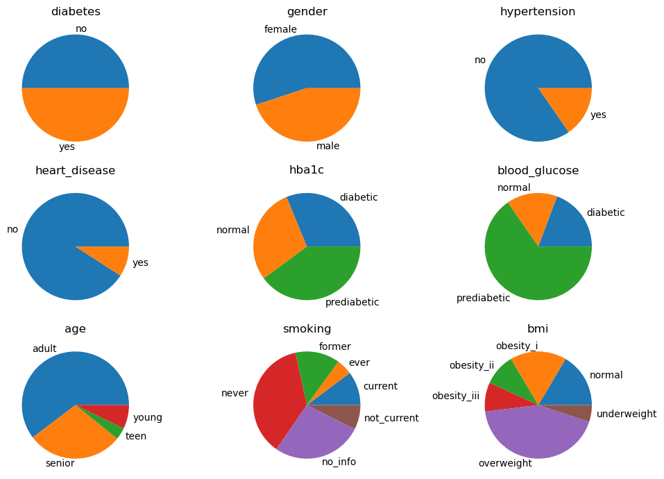
NB, Posteriors
We print the posteriors of the NB model if you are interested.
[10]:
from pysparkbbn.discrete.bbn import get_bbn
from pybbn.pptc.inferencecontroller import InferenceController

bbn = get_bbn(g, p, data.get_profile())
join_tree = InferenceController.apply(bbn)
nb_tree = join_tree
[12]:
import numpy as np
import matplotlib.pyplot as plt

posteriors = join_tree.get_posteriors()

fig, axes = plt.subplots(3, 3, figsize=(10, 7))

for ax, (node, p) in zip(np.ravel(axes), posteriors.items()):
    pd.Series(p).plot(kind='pie', ax=ax)
    ax.set_title(f'{node}')
    ax.set_ylabel('')

fig.tight_layout()
NB, lift
In this type of lift analysis, we want to see which node at its extreme value gives the highest lift to diabetes. Keep an eye on the blood_glucose variable as setting it to yes makes diabetes absolutely certain (100%).
[13]:
from pybbn.graph.jointree import EvidenceBuilder

def get_sensitivity(name, value):
    join_tree.unobserve_all()

    ev = EvidenceBuilder() \
        .with_node(join_tree.get_bbn_node_by_name(name)) \
        .with_evidence(value, 1.0) \
        .build()
    join_tree.set_observation(ev)

    meta = {'name': name, 'value': value}
    post = join_tree.get_posteriors()['diabetes']

    return {**meta, **post}

n2v = {
    'hypertension': 'yes',
    'heart_disease': 'yes',
    'gender': 'male',
    'hba1c': 'diabetic',
    'blood_glucose': 'diabetic',
    'age': 'senior',
    'smoking': 'current',
    'bmi': 'obesity_iii'
}

nb_sen = pd.DataFrame([get_sensitivity(name, value) for name, value in n2v.items()]) \
    .assign(lift=lambda d: d['yes'] / 0.5) \
    .sort_values(['lift'], ascending=False) \
    .rename(columns={'lift': 'diabetes_lift'})

nb_sen
[13]:
| name | value | no | yes | diabetes_lift | |
|---|---|---|---|---|---|
| 4 | blood_glucose | diabetic | 0.000000 | 1.000000 | 2.000000 |
| 3 | hba1c | diabetic | 0.139837 | 0.860163 | 1.720327 |
| 1 | heart_disease | yes | 0.172166 | 0.827834 | 1.655667 |
| 0 | hypertension | yes | 0.194220 | 0.805780 | 1.611560 |
| 7 | bmi | obesity_iii | 0.212166 | 0.787834 | 1.575668 |
| 5 | age | senior | 0.269892 | 0.730108 | 1.460217 |
| 6 | smoking | current | 0.447857 | 0.552143 | 1.104287 |
| 2 | gender | male | 0.468063 | 0.531937 | 1.063873 |
Tree
Now we will learn a MWST model.
Tree, structure learning
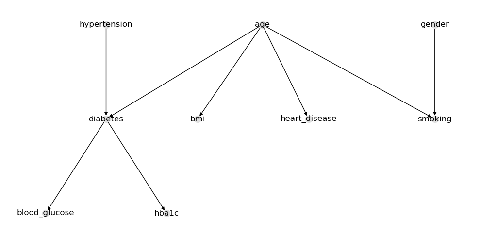
Nothing interesting here except that diabetes and heart_disease have arcs going into age. We will reverse these arcs going the other way.
[14]:
from pysparkbbn.discrete.scblearn import Mwst

data = DiscreteData(sdf)
mwst = Mwst(data)
g = mwst.get_network()

print('')
print('nodes')
print('-' * 10)
for n in g.nodes():
    print(f'{n}')

print('')
print('edges')
print('-' * 10)
for pa, ch in g.edges():
    print(f'{pa} -> {ch}')
23/09/10 17:42:41 WARN CacheManager: Asked to cache already cached data.
nodes
----------
diabetes
blood_glucose
hba1c
age
hypertension
bmi
smoking
heart_disease
gender

edges
----------
diabetes -> blood_glucose
diabetes -> hba1c
diabetes -> age
age -> bmi
age -> smoking
hypertension -> diabetes
heart_disease -> age
gender -> smoking
Since the object instance returned from the algorithm is a networkx graph, it’s easy to do graph surgery (like remove and adding arcs). Just be careful to not introduce cycle. In this case, we were lucky that reversing the arcs did not introduce cycles. In most typical cases, graph surgery will introduce directed cycles.
[15]:
g.remove_edge('diabetes', 'age')
g.remove_edge('heart_disease', 'age')
g.add_edge('age', 'diabetes')
g.add_edge('age', 'heart_disease')
The MWST learned looks reasonable.
[16]:
import networkx as nx
import matplotlib.pyplot as plt

pos = nx.nx_pydot.graphviz_layout(g, prog='dot')

fig, ax = plt.subplots(figsize=(10, 5))

nx.draw(g, pos, ax=ax, with_labels=True, node_size=100, node_color='#e0e0e0')

fig.tight_layout()
Tree, parameter learning
Nothing interesting here; we are just learning the MWST parameters.
[17]:
param_learner = ParamLearner(data, g)
p = param_learner.get_params()
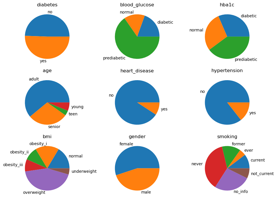
Tree, posteriors
The posteriors of the MWST model is printed below.
[18]:
# create the BBN and Join Tree

bbn = get_bbn(g, p, data.get_profile())
join_tree = InferenceController.apply(bbn)
mwst_tree = join_tree
[19]:
posteriors = join_tree.get_posteriors()

fig, axes = plt.subplots(3, 3, figsize=(10, 7))

for ax, (node, p) in zip(np.ravel(axes), posteriors.items()):
    pd.Series(p).plot(kind='pie', ax=ax)
    ax.set_title(f'{node}')
    ax.set_ylabel('')

fig.tight_layout()
Tree, lift
Let’s compare the lift analysis of the NB and MWST models. Here are some observations.
blood_glucose provides the most lift to diabetes
in the NB model, age ranks pretty high, but in the MWST model, age is near the bottom
smoking and gender do not provide much lift to diabetes
[20]:
mwst_sen = pd.DataFrame([get_sensitivity(name, value) for name, value in n2v.items()]) \
    .assign(lift=lambda d: d['yes'] / 0.5) \
    .sort_values(['lift'], ascending=False) \
    .rename(columns={'lift': 'diabetes_lift'})
mwst_sen
[20]:
| name | value | no | yes | diabetes_lift | |
|---|---|---|---|---|---|
| 4 | blood_glucose | diabetic | 0.000000 | 1.000000 | 2.000000 |
| 3 | hba1c | diabetic | 0.137192 | 0.862808 | 1.725616 |
| 0 | hypertension | yes | 0.229637 | 0.770363 | 1.540726 |
| 5 | age | senior | 0.281937 | 0.718063 | 1.436127 |
| 1 | heart_disease | yes | 0.372553 | 0.627447 | 1.254893 |
| 7 | bmi | obesity_iii | 0.474390 | 0.525610 | 1.051220 |
| 6 | smoking | current | 0.487581 | 0.512419 | 1.024838 |
| 2 | gender | male | 0.494459 | 0.505541 | 1.011082 |
[21]:
nb_sen
[21]:
| name | value | no | yes | diabetes_lift | |
|---|---|---|---|---|---|
| 4 | blood_glucose | diabetic | 0.000000 | 1.000000 | 2.000000 |
| 3 | hba1c | diabetic | 0.139837 | 0.860163 | 1.720327 |
| 1 | heart_disease | yes | 0.172166 | 0.827834 | 1.655667 |
| 0 | hypertension | yes | 0.194220 | 0.805780 | 1.611560 |
| 7 | bmi | obesity_iii | 0.212166 | 0.787834 | 1.575668 |
| 5 | age | senior | 0.269892 | 0.730108 | 1.460217 |
| 6 | smoking | current | 0.447857 | 0.552143 | 1.104287 |
| 2 | gender | male | 0.468063 | 0.531937 | 1.063873 |
If we do a cross tabulation between diabetes and blood_glucose, we see that people with diabetes never have a normal blood_glucose; they always have a prediabetic or diabetic blood_glucose! Likewise, people without diabetes never have diabetic blood_glucose. No wonder this problem is seemingly simple.
[22]:
pd.crosstab(Xy_tr['blood_glucose'], Xy_tr['diabetes'])
[22]:
| diabetes | no | yes |
|---|---|---|
| blood_glucose | ||
| normal | 2347 | 0 |
| prediabetic | 5303 | 4698 |
| diabetic | 0 | 2952 |
Validation
Now let’s validate the NB and MWST models with the testing fold. We will be measuring peformance using Area Under the Curve (AUC) for the Receiver Operating Characteristic (ROC) and Precision-Recall (PR) curves.
[23]:
def get_evidence(name, value, model):
    ev = EvidenceBuilder() \
        .with_node(model.get_bbn_node_by_name(name)) \
        .with_evidence(value, 1.0) \
        .build()
    return ev

def get_evidences(data, model):
    return [get_evidence(name, value, model) for name, value in data.items() if name != 'diabetes']

def infer(data, model):
    model.unobserve_all()
    evidences = get_evidences(data, model)
    model.update_evidences(evidences)
    post = model.get_posteriors()['diabetes']

    return post['yes'], data['diabetes']
[24]:
nb_pred = [infer(data, nb_tree) for data in Xy_te.to_dict(orient='records')]
[25]:
mwst_pred = [infer(data, mwst_tree) for data in Xy_te.to_dict(orient='records')]
These are the performances for the NB model.
[26]:
from sklearn.metrics import roc_auc_score, average_precision_score

_y = pd.DataFrame(nb_pred, columns=['y_pred', 'y_true']) \
    .assign(y_true=lambda d: d['y_true'].map({'yes': 1, 'no': 0}))

pd.Series([
    roc_auc_score(_y['y_true'], _y['y_pred']),
    average_precision_score(_y['y_true'], _y['y_pred'])
], ['AUC_ROC', 'AUC_PR'])
[26]:
AUC_ROC    0.948330
AUC_PR     0.951899
dtype: float64
These are the performances for the MWST model.
[27]:
_y = pd.DataFrame(mwst_pred, columns=['y_pred', 'y_true']) \
    .assign(y_true=lambda d: d['y_true'].map({'yes': 1, 'no': 0}))

pd.Series([
    roc_auc_score(_y['y_true'], _y['y_pred']),
    average_precision_score(_y['y_true'], _y['y_pred'])
], ['AUC_ROC', 'AUC_PR'])
[27]:
AUC_ROC    0.941170
AUC_PR     0.939788
dtype: float64
Interestingly, the NB model does marginally better in terms of both the area under the curve (AUC) for the Receiver Operating Characteristic (ROC) and Precision-Recall (PR) curves.
How does age impact diabetes?
[28]:
def get_node_impact(name, value, model):
    model.unobserve_all()
    model.update_evidences([get_evidence(name, value, nb_tree)])
    p = model.get_posteriors()['diabetes']['yes']
    return {'name': name, 'value': value, 'p': p}

def get_impact(name, model):
    return pd.DataFrame([get_node_impact(name, value, nb_tree)
                         for value in X_tr[name].unique()]) \
        .assign(lift=lambda d: d['p'] / 0.5) \
        .sort_values(['lift'], ascending=False)
If we observe a person classified as a senior, then the probability of having diabetes is 73%.
[29]:
get_impact('age', mwst_tree)
[29]:
| name | value | p | lift | |
|---|---|---|---|---|
| 1 | age | senior | 0.730108 | 1.460217 |
| 0 | age | adult | 0.469881 | 0.939762 |
| 3 | age | teen | 0.092896 | 0.185792 |
| 2 | age | young | 0.029170 | 0.058341 |
How does gender impact diabetes?
Gender does not seem to impact whether one has diabetes or not.
[30]:
get_impact('gender', mwst_tree)
[30]:
| name | value | p | lift | |
|---|---|---|---|---|
| 0 | gender | male | 0.531937 | 1.063873 |
| 1 | gender | female | 0.473953 | 0.947906 |
How does BMI impact diabetes?
As a person’s BMI increases, this increase of BMI also increases the probability of diabetes.
[31]:
get_impact('bmi', mwst_tree)
[31]:
| name | value | p | lift | |
|---|---|---|---|---|
| 0 | bmi | obesity_iii | 0.787834 | 1.575668 |
| 4 | bmi | obesity_ii | 0.733740 | 1.467480 |
| 2 | bmi | obesity_i | 0.634202 | 1.268405 |
| 3 | bmi | overweight | 0.459665 | 0.919330 |
| 1 | bmi | normal | 0.308485 | 0.616971 |
| 5 | bmi | underweight | 0.068299 | 0.136598 |
How does heart disease impact diabetes?
Observing a person with heart disease increases the probability of having diabetes to 83%.
[32]:
get_impact('heart_disease', mwst_tree)
[32]:
| name | value | p | lift | |
|---|---|---|---|---|
| 1 | heart_disease | yes | 0.827834 | 1.655667 |
| 0 | heart_disease | no | 0.467136 | 0.934273 |
How does smoking status impact diabetes?
It looks like if a person was a former smoker, then that increases their probability of having diabetes. Here’s an attempt to explain this observation. People who have quit smoking tend to gain weight because instead of doing the bad habit of smoking, they have replace it with the bad habit of snacking and overeating; hence, former smokers eat more and probably less healthily so, and as a result, increase their probability of diabetes.
[33]:
get_impact('smoking', mwst_tree)
[33]:
| name | value | p | lift | |
|---|---|---|---|---|
| 2 | smoking | former | 0.691033 | 1.382066 |
| 4 | smoking | not_current | 0.557435 | 1.114871 |
| 3 | smoking | ever | 0.553741 | 1.107483 |
| 1 | smoking | current | 0.552143 | 1.104287 |
| 0 | smoking | never | 0.537944 | 1.075889 |
| 5 | smoking | no_info | 0.310254 | 0.620508 |